TL;DR
기존 hyper connection은 residual connection을 대체하여 좋은 성능을 보이지만, 훈련 불안정성 및 메모리 오버헤드가 크다는 단점을 가짐. 이는 hyper connection이 identity mapping을 손상시키기 때문에 일어나는 현상인데, $m$HC는 identity mapping을 복원하면서도 최적화를 통해 효율성을 보장하는 프레임워크를 제안함.
26년 1월 초 가장 핫한 논문중 하나.
- Paper: $m$ HC: Manifold-Constrained Hyper-Connections
- Paper from
Arxiv_2025
🔗 Hyper Connections?
Hyper Connections은 기존 Residual Connection을 발전시킨 개념 (ICLR 2025 D. Zhu. et. al.)
Residual Connection은 단순 합 연산 (Vanishing Gradient 방지)
이에 반해 Hyper Connection은 복잡한 형태로 이뤄짐 (Representation 증대)
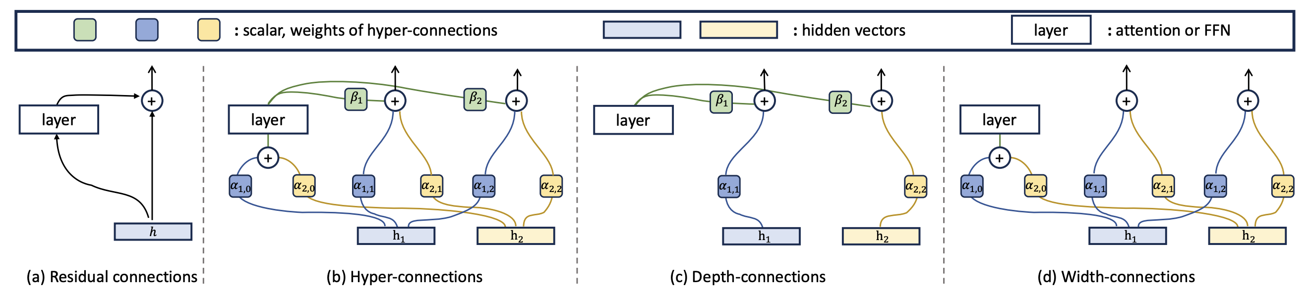
- Depth Connection: residual의 비율을 조절하는 $\alpha$와 $\beta$ 파라미터를 사용.
- Width Connection: 복수의 hidden vectors에 대한 합 연산의 비율을 조절하는 $\alpha$ 파라미터 사용.
- Hyper Connection: Depth + Width Connection, 즉 다양한 합연산 실행시 비율을 조절하는 파라미터들을 사용. 또한 layer 입력에 대한 비율 조절도 가능.
모델이 이전 입력의 영향력을 줄이고 싶을 때 학습을 통해 이를 실현 가능함.
다만 훈련 강도가 높아짐에 따라 (Large-scale training) 학습의 불안정성이 높아질 수 있는데, 이는 Identity 보존이 힘들기 때문이라고 함. 여러 layer를 거치며 Residual Connection은 이전 입력을 일정하게 합하며 원본 feature를 보존할 수 있는데, HC는 $\alpha, \beta$가 줄어들거나 커질 때 그만큼 layer별로 원본이 훼손되거나 학습이 제대로 안되는 등 complexity가 높아짐 + Hardware issue.
예를 들어 매 층마다 1.1배씩 신호를 키운다고 하면, 100번째 층에서는 $1.1^{100} \approx 13,780$배
수식으로 표현하면 다음과 같다 (복수의 feature가 아닌 단일 feature 상황):
각 변수는 다음과 같이 정의할 수 있다:
- $\alpha$는 값의 크기를 조절하는 learnable gating factor를 의미
- $\theta$는 projection parameter
- $b$는 learnable bias
- $x_l\in\mathbb{R}^{n\times C}$
- $\theta^{pre}, \theta^{post} \in \mathbb{R}^{1\times C}, \theta^{res}\in\mathbb{R}^{n\times C}$
- $b^{pre}, b^{post} \in \mathbb{R}^{1\times n}, b^{res} \in \mathbb{R}^{n \times n}$
즉, 각 layer마다 연산이 recursive하므로, 식을 다음과 같이 전개 할 수 있음.
$\mathcal{H}^{\text{res}}$는 결국 앞서 말한것처럼 recursive 되며 값이 폭발하거나 없어지는 현상 발생
🐳 Manifold-Constrained Hyper-Connections ($m$HC)
HC는 실제로 성능이 좋지만, layer가 깊어짐에 따라 불안정한 학습과 큰 오버헤드가 단점
$m$HC: 오버헤드를 줄이고, 안정적인 학습을 위해 최적화 테크닉을 적용해보자!
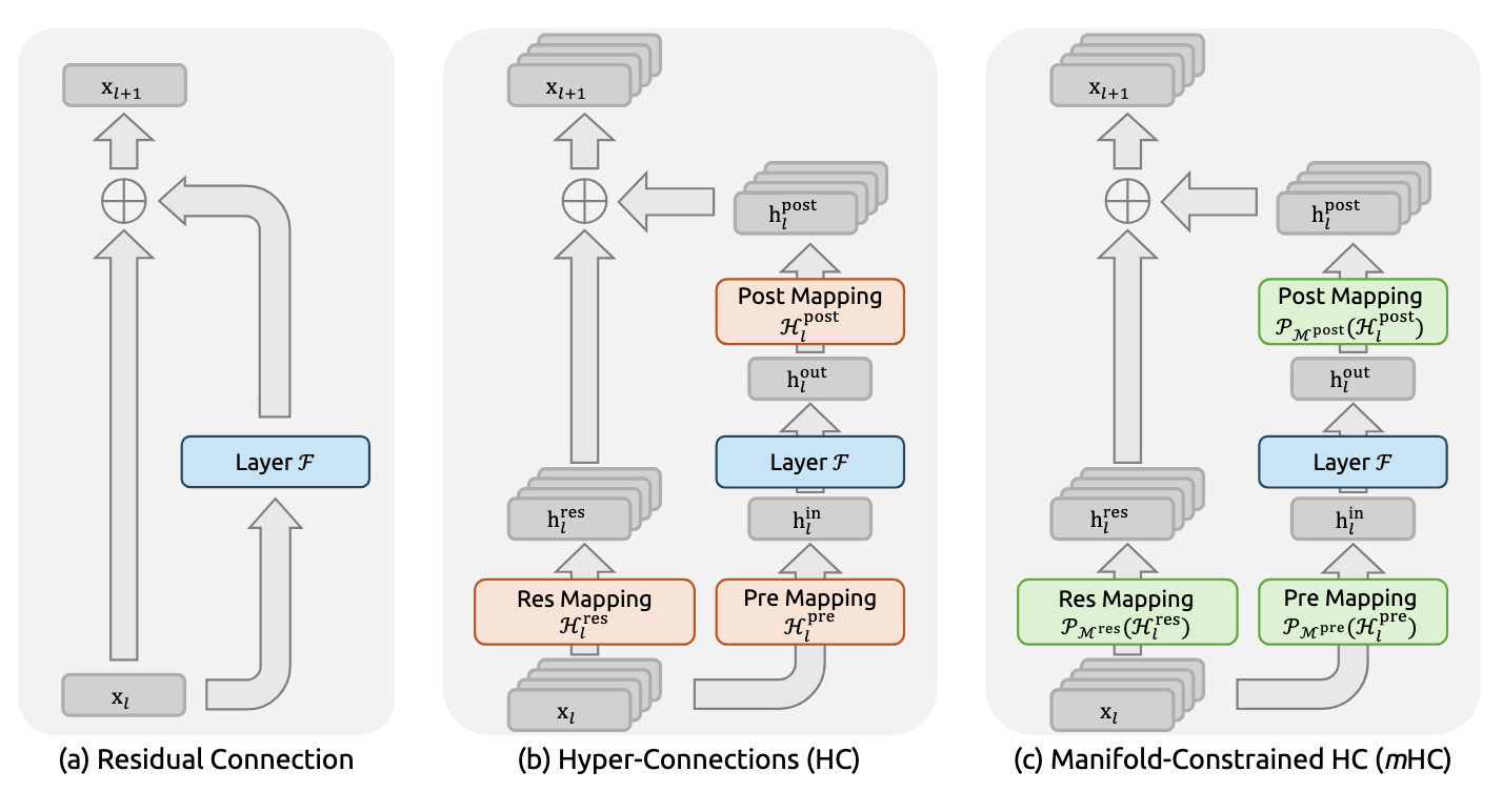
가장 핵심적인 부분은 $\mathcal{H}^{\text{res}}$의 증폭 크기를 줄이는것 (Gain Magnitude)
기존 HC는 layer가 깊어짐에 따라 최대 3000까지 치솟는 것을 확인
$m$HC는 $\mathcal{H}^{\text{res}}$를 doubly stochastic matrix(이중 확률 행렬)로 강제하여 증폭을 해결 –> 이를 manifold에 투영한다고 표현한 듯
Doubly stochastic matrix: 모든 원소가 음수가 아니며, 각 행의 합과 각 열의 합이 모두 1인 정사각 matrix
Doubly stochastic matrix끼리는 서로 곱했을 때 결과가 doubly stochastic matrix가 된다는 특징이 있음
이를 통해 얻을 수 있는 이점은 다음과 같음.
- Norm Preservation: $\bigg( \prod^{L-1}_{i=1} \mathcal{H}^{\text{res}}_{L-i} \bigg) x_{l}$은 계속해서 행과 열의 합이 1이 되기 때문에 Spectral Norm이 1로 제한되어 gradient exploding을 방지 할 수 있음
- Compositional Closure: 여러 layer에 걸쳐 확률적으로 유지되는 특징 덕분에 모델의 깊이 측면에서 stability를 유지할 수 있음
- Geometric Interpretation via the Birkhoff Polytope: $\mathcal{H}^{\text{res}}$의 집합은 convex hull인 Birkhoff polytope를 형성하는데, 기하학적으로 이같은 조합은 반복적으로 적용 시 정보혼합이 단조롭게 증가하는 경향이 있어 feature fusion mechanism에 적합함
추가적으로 $\mathcal{H}^{\text{pre}}_{l}$과 $\mathcal{H}^{\text{post}}_{l}$에도 비음수가 되도록 제약(sigmoid)을 걸어 양의 계수와 음의 계수의 합성으로 인해 발생하는 signal cancellation을 방지하였음
🗺️ Parameterization and Manifold Projection
위의 방법의 실제 적용을 위해 사용한 방법을 설명
먼저 l-th layer 입력 $x_l \in \mathbb{R}^{n\times C}$를 flatten 한 vector $\vec{x}=\text{vec}(x_l)\in\mathbb{R}^{1\times nC}$ 에 대한 HC fomulation은 다음과 같이 정리가 가능
$\varphi$는 dynamic projection을 위한 linear projection을 나타내며, $\text{mat}(\cdot)$은 flatten된 vector의 공간을 복원하는 매소드. 이때 실제 적용하는 $\mathcal{H}$는 다음과 같이 정의 됨:
즉 pre, post는 sigmoid로 비음수 제약 / res는 sinkhorn-Knopp 알고리즘을 통해 doubly stochasitc matrix로 변환 함.
해당 수식은 $M^{(0)}=\exp(\tilde{\mathcal{H}}_l^{res})$ 부터 시작해서, 각 행과 열을 t번 번갈아 가며 normalization을 진행하는 형태
이때 $t_{\max} \rightarrow \infty$ 일때 결국 어느 시점에서 수렴하여 행과 열의 합이 1인 doubly stochasitc matrix로 변환되며, 현실적으로 너무 큰 반복은 불가능하므로 $t_{\max}=20$으로 사용하였음